
In February 2015, Kaspersky Labs released a report (PDF) detailing its investigation into the Equation Group, an extremely sophisticated hacker group engaged in espionage. Many experts suspect the United States’ NSA to be behind Equation Group due to keywords identified in malware the group has produced. In this article, I will use a different approach to produce evidence for attribution. Kaspersky released, in addition to it’s initial report, data on the dates that pieces of malware were compiled by Equation Group. These timestamps fall almost exclusively during the working week and appear to follow a 9:00 to 5:00 schedule. Assuming that Equation Group is operated by a state actor (government), we can correlate these dates with holidays to identify countries that are more or less likely to be responsible.
Summary
For those of you who want to skip the details, here’s the lowdown. If Equation Group randomly chooses weekdays to compile their programs, but skips most national holidays in whatever country they’re from, then we can use the EquationDrug timestamps to help us figure out who’s responsible. EquationDrug is the name given to the software platform developed by the Equation Group. Each component of EquationDrug includes a timestamp that indicates when it was produced. First, we download all the national holidays for several possible culprits (countries). Then, we simulate 10,000 random sets of weekdays that imitate “timestamps” that Equation Group could have chosen. For every country, we calculate how many of these days fall on national holidays. Then, we compare that to how many of the true Equation Group dates actually fell on that country’s holidays. For some countries, like Brazil, the average (expected) number of holiday timestamps is almost identical to the true number of timestamps observed on holidays. For other countries, like the United States, we expect to see roughly three timestamps on holidays but actually see only one. In fact, only about 20% of the simulated sets of timestamps contain only one or zero holidays for the United States. In other words, if Equation Group randomly chose days to compile their malware, there is only a one in five chance they’d have overlapped with as few U.S. holidays as they did. While this is not a smoking gun, it does place the USA in the top three “most likely” suspects of 79 potential countries. The other two are South Korea and Barbados. It is by far the “most likely” culprit among some of the world’s best cyber powers (including Russia, China, Iran, Israel, and the UK).
The code for reproducing this analysis is available in full below and also on my github. To reproduce this analysis, you will need R and several packages including XML, knitr, timeDate, and stringr.
Getting Data
First, we will download holiday data for several candidate countries from timeanddate.com. To do this, we’ll use the XML package in R. There are 79 candidate countries for which holiday data is available from 2001 to 2013. The remaining countries are omitted from consideration because holiday data is not available for the full range of dates.
library(timeDate)
library(XML)
library(stringr)

# Get a list of available countries from timeanddate.com.
base.url <- "http://www.timeanddate.com"
holidays.url <- "http://www.timeanddate.com/holidays"
page <- htmlParse(holidays.url)
links <- str_extract_all(toString.XMLNode(page),'/holidays/[^/|^\"]+')[[1]]
countries <- gsub("/holidays/","",links)
countries <- countries[!duplicated(countries)]

parseHolidays <- function(yy,cc,base.url)
{
  # Args:
  #   yy: The desired year in yyyy format.
  #   cc: The desired country name from www.timeanddate.com.
  #   base.url: The base url string http://www.timeanddate.com/holidays.
  #
  # Returns:
  #   A dataframe of national holidays for that country year.

  holiday.url <- paste(base.url,cc,yy,sep="/")
  page <- htmlParse(holiday.url)
  tabs <- readHTMLTable(page, header=T)
  holiday.table <- tabs[[1]]
  holiday.table <- holiday.table[grepl("National holiday|Bank holiday|Public Holiday|Feriado Nacional",
                                       holiday.table[,4],ignore.case=T),]
  date <- paste(holiday.table[,1],yy,sep=" ")
  date <- as.Date(date, "%b %d %Y")
  name <- holiday.table[,3]
  holidays <- list(data.frame("date"=date,"name"=name,"country"=cc))
  return(holidays)
}

# For every year and every country, call timeanddate.com to get holidays.
years <- 2001:2013
holiday.list <- list()
for(yy in years)
{
  for(cc in countries)
  {
    try(holiday.list <- c(holiday.list,parseHolidays(yy,cc,holidays.url)))
    Sys.sleep(runif(1,0.25,1))
  }
}

# Turn holiday data into a list of country-based dataframes.
# Yes, this code is a total mess.
holiday.df <- do.call(rbind,holiday.list)
holiday.list <- split(holiday.df, holiday.df$country)
holiday.list <- holiday.list[
  unlist(
    lapply(holiday.list,FUN=function(x)all(2001:2013%in%unique(format(x$date,"%Y")))))]
Next, we’ll load the Equation Group’s link timestamp dates into the R object eq.dates. These come from Kaspersky Labs. The three weekend dates observed in the Equation Group’s timestamps are thrown out and our analysis assumes that the remaining weekdays are chosen at random. This is due to the fact that we have to make assumptions about the data generating process and cannot infer the day-of-week distribution from the observed data without risking post-treatment bias. Simply put, it is easiest (and, in my opinion, safest) to assume that the three weekend timestamps are outliers regardless of the country in which Equation Group is operating and that the distribution of weekday timestamps is random and uniform (controlling for holidays).
# Load all the EquationDrug dates given by Kaspersky.
eq.dates <- c("2001.08.17", "2007.12.11", "2009.04.16", "2011.10.20", "2012.08.31", "2013.06.11",
"2001.08.23", "2007.12.17", "2009.06.05", "2011.10.26", "2012.09.28", "2013.06.26",
"2003.08.16", "2008.01.01", "2009.12.15", "2012.03.06", "2012.10.23", "2013.08.09",
"2003.08.17", "2008.01.23", "2010.01.22", "2012.03.22", "2012.11.02", "2013.08.28",
"2005.03.16", "2008.01.24", "2010.02.19", "2012.04.03", "2012.11.06", "2013.10.16",
"2005.09.08", "2008.01.29", "2010.02.22", "2012.04.04", "2013.01.08", "2013.11.04",
"2006.06.15", "2008.01.30", "2010.03.27", "2012.04.05", "2013.02.07", "2013.11.26",
"2006.09.18", "2008.04.24", "2010.06.15", "2012.04.12", "2013.02.21", "2013.12.04",
"2006.10.04", "2008.05.07", "2011.02.09", "2012.07.02", "2013.02.22", "2013.12.05",
"2006.10.16", "2008.05.09", "2011.02.23", "2012.07.09", "2013.02.27", "2013.12.13",
"2007.07.12", "2008.06.17", "2011.08.08", "2012.07.17", "2013.04.16",
"2007.10.02", "2008.09.17", "2011.08.30", "2012.08.02", "2013.05.08",
"2007.10.16", "2008.09.24", "2011.09.02", "2012.08.03", "2013.05.14",
"2007.12.10", "2008.12.05", "2011.10.04", "2012.08.14", "2013.05.24")
eq.dates <- as.Date(eq.dates,"%Y.%m.%d")
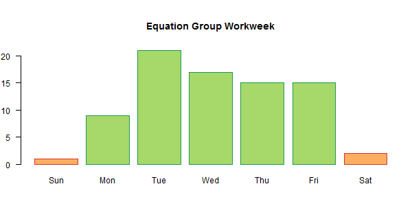
# Plot the workweek of Equation Group.
eq.week <- table(dayOfWeek(timeDate(eq.dates)))
par(mar=c(4.1,2.1,5.1,1.1),mfrow=c(1,1))
bar.color <- c("#fdae61",rep("#a6d96a",5),"#fdae61")
lin.color <- c("#d73027",rep("#1a9850",5),"#d73027")
barplot(eq.week[c("Sun","Mon","Tue","Wed","Thu","Fri","Sat")],
col=bar.color, border=lin.color,
main="Equation Group Workweek", las=1)
# Remove weekends from the Equation Group dates.
eq.dates <- eq.dates[isWeekday(eq.dates)]
Methodology
Now that we have the Equation Group data and data on national holidays for several potential nation-state culprits, we can determine which countries are more or less likely to have sponsored Equation Group. There are a few important assumptions to be made first:
- Link dates for EquationDrug malware are randomly chosen from the work week.
- Equation Group observes, in general, official holidays of the state in which they operate.
- The timestamps given by Kaspersky are accurate. (Note that there are many reasons that this assumption could be wrong. First, Equation Group could obscure the timestamps. More importantly, the computer's time zone might not match the programmer's time zone. Unfortunately, without the full timestamp data for each piece of malware, I cannot think of a way to compensate adequately for this.)
The code below sets parameters and then simulates 10,000 sets of dates of the same size (and during the same time period) as the dates given by Kaspersky. Then, it cycles through each country’s list of holidays and calculates how many of the simulated dates and the observed (Kaspersky) dates fall on that country’s holidays.
# Set parameters
all.dates <- seq(min(eq.dates),max(eq.dates),by=1)
all.dates <- all.dates[isWeekday(all.dates)]
n <- 10000

# Simulate n link dates
sample.dates <- list()
for(ii in 1:n)
{
  week.sample <- sample(all.dates, length(eq.dates), replace=F)
  sample.dates <- c(sample.dates, list(week.sample))
}

# Calculate holiday distribution for each country
simulated.list <- list()
observed.list <- NULL
country.name <- NULL
for(cc in holiday.list)
{
  simulated.list <- c(simulated.list, list(lapply(sample.dates, FUN=function(x){sum(x %in% cc$date)})))
  observed.list <- c(observed.list, sum(eq.dates %in% cc$date))
  country.name <- c(country.name,as.character(unique(cc$country)))
}
Results
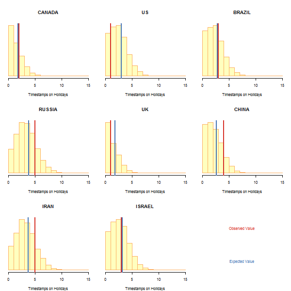
First, we will look at a select group of possible countries behind Equation Group. These include the world’s most sophisticated cyber powers and a couple additional countries from the UTC-3 timezone (which matches the observed hourly distribution of timestamps given by Kaspersky). The plots above show the simulated distribution of holidays worked by Equation Group when their work days are chosen at random (yellow). The red bar indicates the actual number of holidays worked by the Equation Group while the blue bar represents the expected number of holidays that would have been worked if days were chosen at random with respect to that country’s holidays.
results.df <- NULL
country.name <- toupper(country.name)
interesting.countries <- c("US","UK","RUSSIA","IRAN","CHINA","BRAZIL","CANADA","ISRAEL")
bar.color <- "#ffffbf"
exp.color <- "#4575b4"
obs.color <- "#d73027"
lin.color <- "#fdae61"

par(mfrow=c(3,3), mar=c(4.1,1.1,5.1,1.1))
for(cc in 1:length(country.name))
{
  c.name <- country.name[cc]
  proportion <- mean(simulated.list[[cc]] <= observed.list[cc])
  expected <- mean(as.numeric(simulated.list[[cc]]))
  results.df <- rbind(results.df, data.frame(Country=c.name,
                                             Probability=proportion,
                                             Observed=observed.list[cc],
                                             Expected=expected,
                                             Difference=observed.list[cc]-expected))
  if(c.name %in% interesting.countries)
  {
    hist(as.numeric(simulated.list[[cc]]),
         breaks=0:max(unlist(simulated.list)),
         col=bar.color, border=lin.color,
         ylab="", xlab="Timestamps on Holidays",
         main=country.name[cc], yaxt="n", yaxs="i")
    abline(v=expected, col=exp.color, lwd=2)
    abline(v=observed.list[cc], col=obs.color, lwd=2)
  }
}
plot(0,0,type="n",xaxt="n",yaxt="n",main="",xlab="",ylab="",xlim=c(-1,1),ylim=c(0,3),frame=F)
text(0,.5,"Expected Value",col=exp.color)
text(0,2.5,"Observed Value",col=obs.color)
Clearly, the United States stands out in that the number of US holidays actually worked by the Equation Group is two lower than the expected number of holidays that would have been worked had Equation Group not observed US holidays. If the Equation Group does not actually follow a US calendar, then one would only expect to see this few holidays worked less than 20% of the time. This indicates that the Equation Group is more likely to follow the US calendar than any of the others examined here. In fact, it puts the United States among the top three countries (of 79) in terms of those that are least likely to have had so few working holidays if the Equation Group were located elsewhere. The top ten least likely to have happened by chance are shown in the table below.
Country       Probability
 SOUTH-KOREA   0.1573
 BARBADOS      0.1736
 US            0.1947
 SLOVENIA      0.2167
 GREECE        0.2214
 LUXEMBOURG    0.2245
 NEW-ZEALAND   0.2290
 LITHUANIA     0.2721
 LIECHTENSTEIN 0.3175
 ITALY         0.3233
In the above table, “Probability” refers to the probability that so few timestamps occurred on holidays in that country if the Equation Group selects workdays at random. Therefore, a low probability implies that it is less likely the dates were chosen at random with respect to that country’s holidays.
print(
head(
results.df[order(results.df$Probability),c("Country","Probability")], 10),
right=F, row.names=F)
Conclusion
This analysis is by no means the smoking gun in Equation Group attribution. However, it does lend credence to the theory that the United States is behind the group and, when combined with the other evidence already provided by Kaspersky, makes a strong case for attribution. By simply comparing the dates worked by Equation Group to a corpus of national holidays, the United States floats to the very top of most likely culprits.