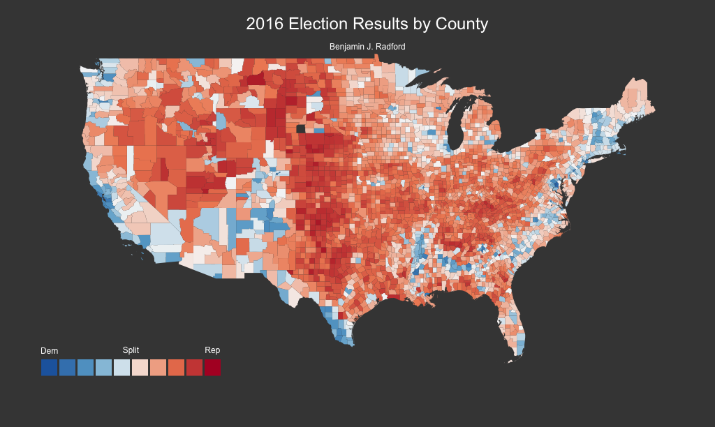
In a shocking turn of events, Donald Trump won the 2016 U.S. presidential election. After the shock (and distress) subsided, some (myself included) were left wondering if this twist ending was the work of hackers manipulating electronic voting machines. It is certainly possible to hack e-voting machines. And there is evidence that a state actor did engage in an effort to manipulate the U.S. election. Putting the two together, some experts have advised the Clinton campaign that votes cast on e-voting machines should be audited for the possibility that these machines were compromised by foreign agents. These experts claim to have found evidence that Trump performed disproportionately well in certain counties where electronic voting machines were used. Nate Silver of 538 disagrees. In this article, I provide the data and code necessary to test this hypothesis and to potentially uncover evidence of manipulated, hacked, or otherwise unfair e-voting machines. While I find no evidence that e-voting machines were biased in favor of either candidate, I encourage others to build on this analysis and verify (or contradict) these results.
All code and data to replicate this analysis can be found at GitHub.com/benradford/electiogeddon.
Data Sources
First, we need to obtain several sets of data. These are listed below and include election returns, voting technology by county, and demographic data. Fortunately, all of these are available online for free and are also available in easy CSV format in this project’s associated GitHub repository. Additionally, all but one source of data use FIPS codes to facilitate merging the disparate sources together.
- Demographic data on race and sex from the U.S. Census Bureau.
- Education data from the U.S. Department of Agriculture.
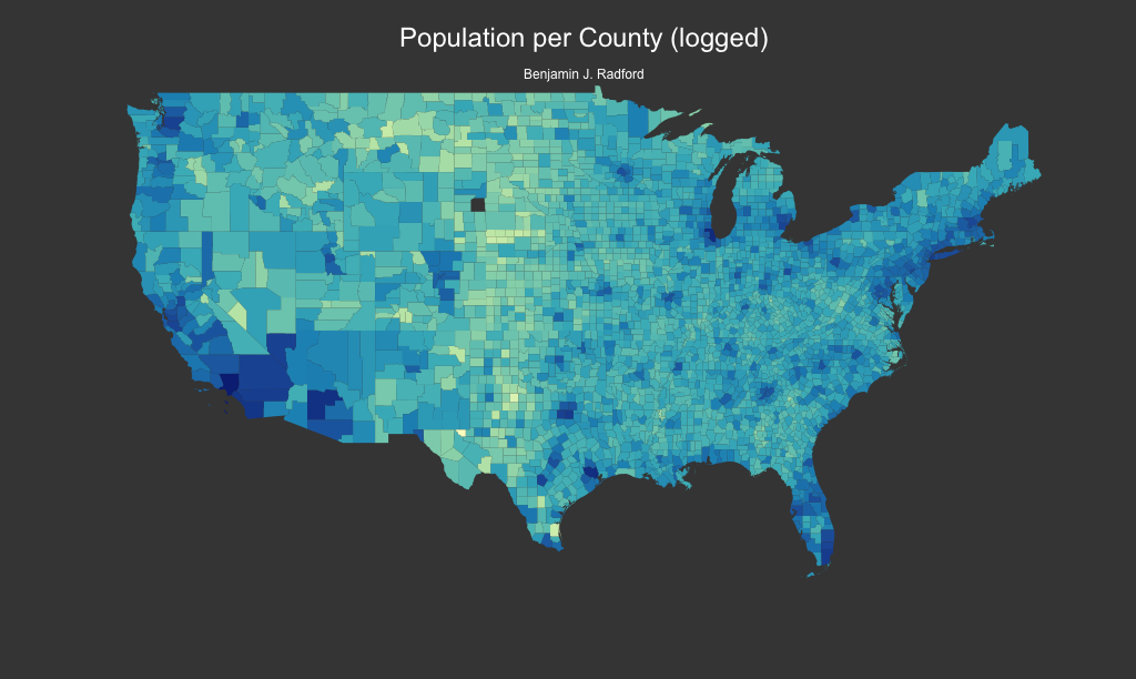
- Population data from the U.S. Department of Agriculture.
- Unemployment data from the U.S. Department of Agriculture.
- 2016 U.S. presidential election results from tonmcg.
- 2016 U.S. presidential election voting technology from VerifiedVoting.org.
- County-level (adm02) shapefile for U.S.A. from the U.S. Census Bureau.
For data merging issues, Alaska is omitted. For ease of visualization, Hawaii is also omitted.
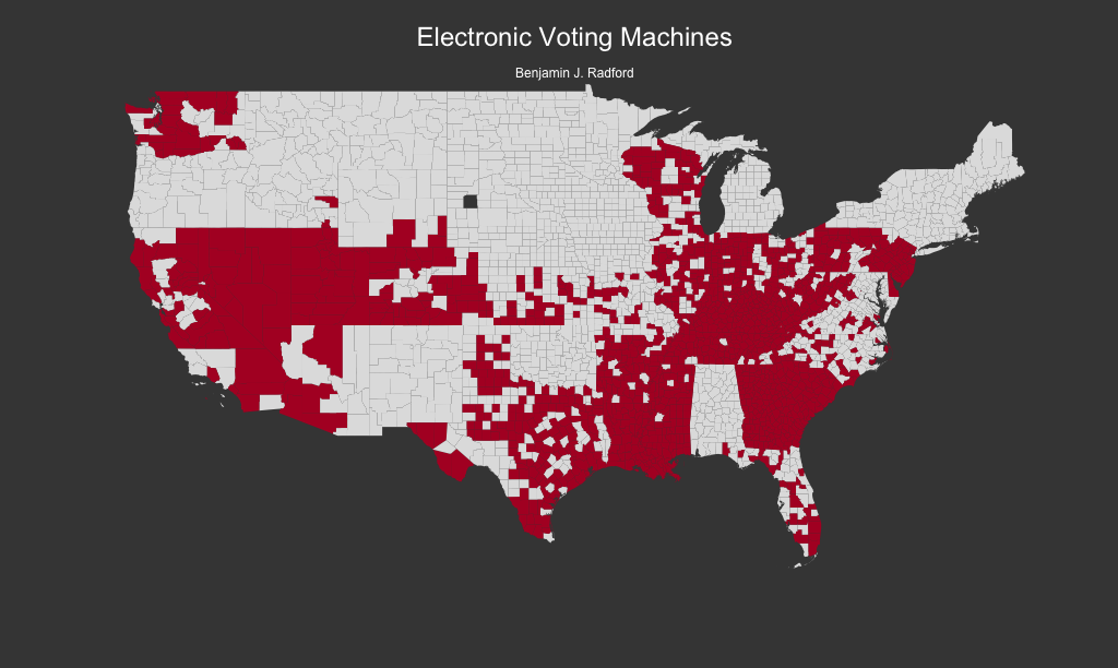
We are testing the hypothesis that, all else considered, counties with electronic voting machines produced vote tallies indistinguishable from those of counties without electronic voting machines. This hypothesis follows from the observation that hackers could manipulate electronic voting machines but could probably not interfere with paper or optical ballots. If we observe a measurable effect of electronic voting machines on the proportion of the vote received by the GOP candidate, we will have evidence to reject the null hypothesis (above) and should consider the possibility that the electronic voting machines were somehow unfair.
The dependent variable is the proportion of vote received by the GOP candidate, Donald Trump, per county. Predictors include electronic voting machines (indicator), population (logged), percent unemployment, percent college degree, and precent white. For simplicity the dependent variable is conceptualized as a continuous-valued response and no link function is used. Therefore, these are purely linear models and predicted values are not bound by 0 and 1 as proportions would be.
| A. GOP Vote Share | B. GOP Vote Share | |||||||
| B | CI | p | B | CI | p | |||
| Fixed Parts | ||||||||
| (Intercept) | 0.62 | 0.59 – 0.66 | <.001 | 0.49 | 0.44 – 0.54 | <.001 | ||
| electronic | 0.01 | -0.00 – 0.03 | .135 | 0.01 | -0.00 – 0.01 | .260 | ||
| population | -0.02 | -0.02 – -0.01 | <.001 | |||||
| unemployment | -0.02 | -0.02 – -0.01 | <.001 | |||||
| college | -0.01 | -0.01 – -0.01 | <.001 | |||||
| percent_white | 0.64 | 0.61 – 0.66 | <.001 | |||||
| Random Parts | ||||||||
| σ2 | 0.018 | 0.007 | ||||||
| τ00, state | 0.014 | 0.007 | ||||||
| Nstate | 49 | 49 | ||||||
| ICCstate | 0.435 | 0.507 | ||||||
| Observations | 3107 | 3105 | ||||||
| R2 / Ω02 | .319 / .319 | .746 / .746 | ||||||
For the national models, linear mixed effects models are selected. Random intercepts are included per state. These allow us to account for state-level heterogeneity; we are essentially controlling for all of the systematic differences between states that are otherwise unaccounted for by the variables in our model. For example, differences between states in geography, state history, and industry should all more-or-less be covered by these higher-level random effects. Neither model A nor B provides evidence of a significant or substantial correlation between voting technology and vote share. This means we have found no evidence to reject the null hypothesis and are still safe to assume that, nationally, electronic voting machines do not correlate with unusual voting behaviors at the county level.
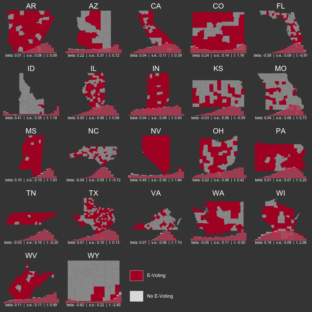
We turn now to a state-level analysis. For this, I have elected to use 22 simple linear regression models - one per state with mixed voting types. Because we need to measure variation within the state, we must omit the remaining states that utilize either electronic voting or other voting methods but not both. Rather than show 22 regression tables, the results are shown here as a series of maps.
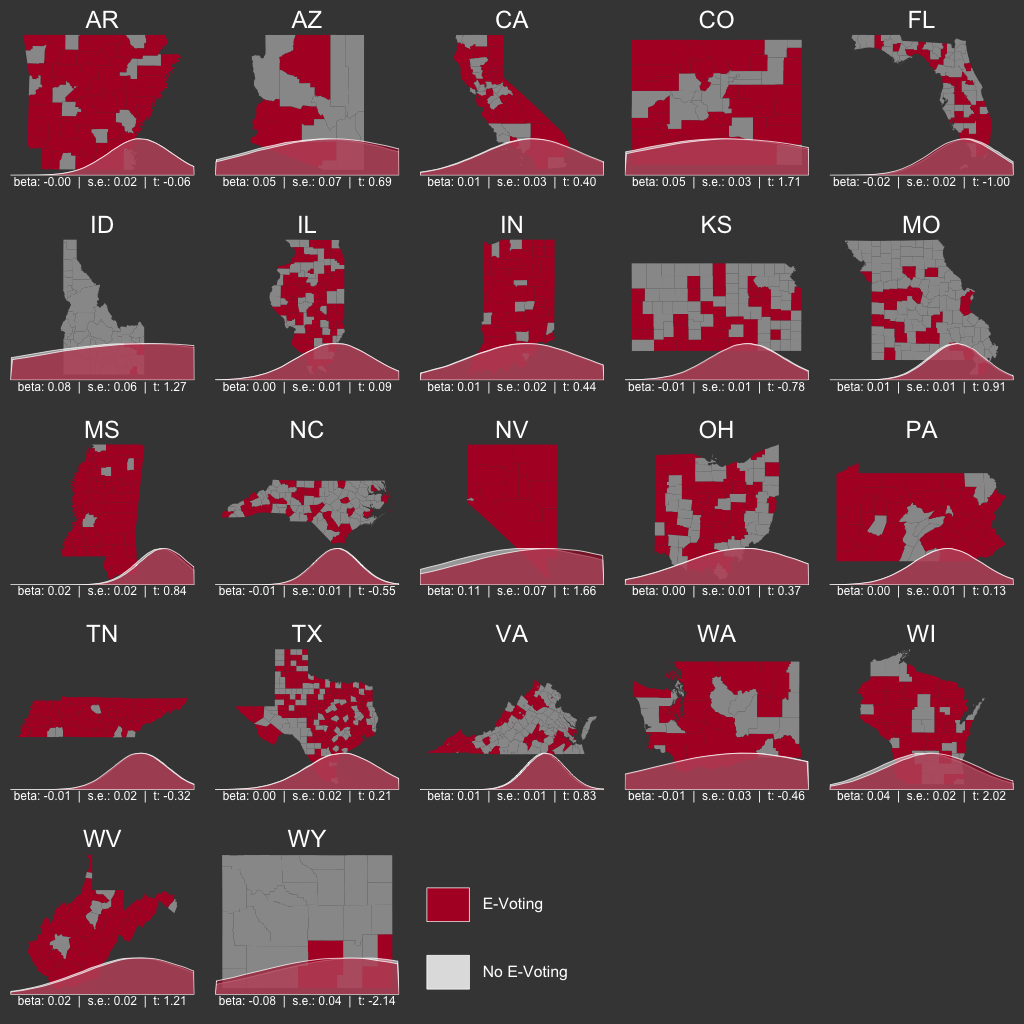
Underneath each state map is a pair of overlapping density plots. These represent the predicted values of GOP vote share given the state model and model uncertainty. If the red (e-voting) and gray (not e-voting) densities overlap, that means the predicted values for vote share in that state are roughly the same for counties that use electronic voting machines and those that do not. If, on the other hand, the two densities do not line up, we would suspect that there are systematic (but otherwise unaccounted for) differences in the e-voting and not e-voting counties in that particular state.
Below the density plots, we see the regression coefficient beta, standard error s.e., and t-score t for that state’s model. In only two of 22 analyzed states is e-voting a significant predictor of vote share at traditional levels of confidence. In Wisconsin counties with e-voting were more likely to lean Trump than Clinton. However, in Wyoming, counties with e-voting leaned Clinton over Trump. Neither of these results holds up to a Bonferroni correction for multiple hypothesis testing and should therefore be viewed skeptically. See the [edit] below for results from an alternative modeling strategy.
Conclusion
This miniature study finds no compelling evidence that electronic voting machines were biased for or against either of the candidates in the 2016 U.S. presidential election. This result agrees with a similar analysis by Nate Silver. However, there are a few caveats:
- It is unlikely that hackers would target all electronic voting machines rather than a particular make or model of machine. Given that each model is likely to run on its own software and contain its own unique vulnerabilities, hackers may be more likely to single out a particular brand or type of voting machine rather than target an entire state’s worth of voting machines. A follow-up analysis should consider machine make and model as a predictor of vote share. Voting machine make and model are included in the provided data.
- Hackers are smart and will cover their tracks well. The fact that county-level vote manipulation is not obvious from this analysis does not mean that vote hacking did not occur. It only means that, if it did, the perpetrators were more clever than I assume here.
I encourage anybody interested in politics and data analysis to replicate and expand on this study. The code and data to get started are available for free here.
Update
Thanks to a good suggestion in the comments from Tracy Carr, I have repeated the state-level analysis using generalized linear models and stipulating a quasi-binomial response variable (proportion of votes received by GOP). I have elected to use a quasi-binomial over a standard binomial distribution to allow the model to account for under or over-dispersion in observed vote proportions from county to county. The results are visualized below. Estimated t-scores and relative predicted values largely mirror those described by the linear models above.
Additionally, I have re-estimated the national-level models. The results are below. Again, these are generalized linear models and an assumed quasi-binomial response. Due to the limitations of my preferred R package for estimated mixed effects models, I have instead opted to use state fixed effects. The fixed effects are omitted here.
Bivariate model
Estimate Std. Error t value Pr(>|t|)
(Intercept)         0.64841    0.07368   8.800  < 2e-16 ***
electronic          0.04608    0.03471   1.328 0.184416

Multiple regression model
Estimate Std. Error t value Pr(>|t|)
(Intercept)         0.6808860  0.1179998   5.770 8.71e-09 ***
electronic          0.0113319  0.0225596   0.502 0.615485
population         -0.0855596  0.0069790 -12.260  < 2e-16 ***
unemployment       -0.0774218  0.0056691 -13.657  < 2e-16 ***
college            -0.0284239  0.0011195 -25.389  < 2e-16 ***
percent_white       0.0285929  0.0006607  43.275  < 2e-16 ***